
Classification of Interpolation Techniques
Interpolation techniques can can be classified in following five main classes:
1. Point Interpolation/Area Interpolation
2. Global/Local Interpolations
3. Exact/Approximate Interpolations
4. Stochastic/Deterministic Interpolations
5. Gradual/Abrupt Interpolations
Point/Line/Area Interpolation
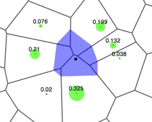
In point interpolation, given a number of points whose locations and values are known, determine the values of other points at predetermined locations. Point interpolation is used for data which can be collected at point locations e.g. weather station readings, spot heights, oil well readings, porosity measurements. Point to point interpolation is the most frequently performed type of spatial interpolation done in GIS.
e.g. Precipitation and rainfall data
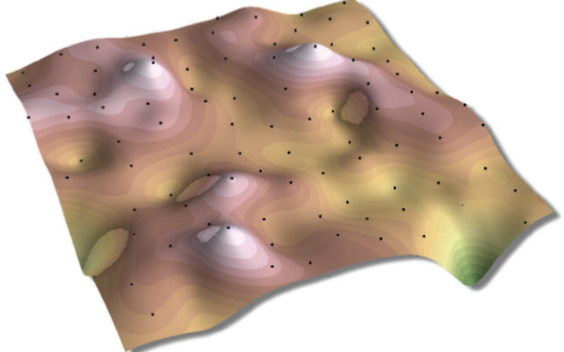
Point Interpolation
The input data does not necessarily need to be points. In fact, points, lines and/or areas can be interpolated. Paper maps often have the elevation represented as isolines, where the elevation is the same along a particular line. If such isolines were digitized, they could be interpolated to create a continuous surface (DEM). But often, isolines are the result of a first interpolation.
e.g: contours to elevation grids
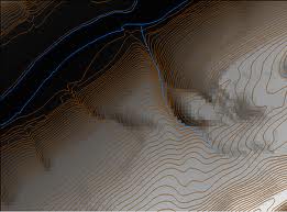
Line Interpolation
The 3rd option, area-based interpolation is not very common, but nevertheless exists. In area-based interpolation, given a set of data mapped on one set of source zones determine the values of the data for a different set of target zones. For example, if one had a population raster showing the number of people per square km, and wanted to estimate the population per municipality, such a method could be used.
e.g: given population counts for census tracts, estimate populations for electoral districts.
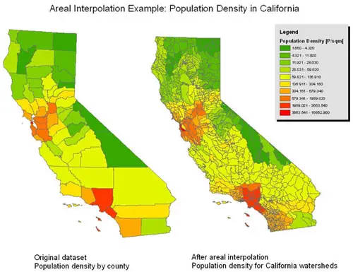
Area Interpolation
Global/Local Interpolations
Global Interpolation methods apply a single mathematical function to all observed data points and generally produce smooth surfaces. A change in one input value affects the entire map. Global Interpolation is used when there is an hypothesis about the form of the surface, e.g. a trend
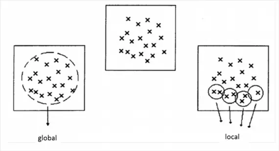
Global and Local Interpolation
Local methods apply a single mathematical function repeatedly to small subsets of the total set of observed data points and then link these regional surfaces to create a composite surface covering the whole study area. A change in an input value only affects the result within the window. Some local interpolators may be extended to include a large proportion of the data points in set, thus making them in a sense global.
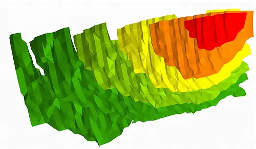
Exact or Approximate Interpolation
Exact methods of point interpolation honour all the observed data points for which data are available. This means that the surface produced passes exactly through the observed data points, and must not smooth or alter their values. Exact methods are most appropriate when there is a high degree of certainly attached to the measurements made at the observed data points.
e.g. proximal interpolators, B-splines and Kriging methods all honor the given data points.
Exact Interpolation
Approximate methods of interpolation do not have to honour the observed data points, but can smooth or alter them to fit a general trend. Approximate methods are more appropriate where there is a degree of uncertainty surrounding the measurements made at the sample points.
Approximate Interpolation
This utilizes the belief that in many data sets there are global trends, which vary slowly, overlain by local fluctuations, which vary rapidly and produce uncertainty (error) in the recorded values. The effect of smoothing will therefore be to reduce the effects of error on the resulting surface.
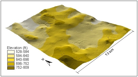
Gradual or Abrupt Interpolation
Gradual and abrupt interpolation methods are distinguished by the continuity of the surface produced. Gradual methods produce a smooth surface between sample points whereas abrupt methods produce surfaces with a stepped appearance. Terrain model may require both methods as it may be necessary to reproduce both gradual changes between observed points, for example in rolling terrain, and abrupt changes where cliffs and valley occur.
A typical example of a gradual interpolater is the distance weighted moving average. Usually produces an interpolated surface with gradual changes. However, if the number of points used in the moving average is reduced to a small number, or even one, there would be abrupt changes in the surface.
Abrupt Interpolation
It may be necessary to include barriers in the interpolation process
- semipermeable, e.g. weather fronts
- will produce quickly changing but continuous values
- impermeable barriers, e.g. geologic faults
- will produce abrupt changes
Deterministic or Stochastic Interpolation
Deterministic methods of interpolation can be used when there is sufficient knowledge about the geographical surface being modeled to allow its character to be described as a mathematical function. Unfortunately, this is rarely the case for surfaces used to represent real-world features. To handle this uncertainty stochastic (random) models are used to incorporate random variation in the interpolated surface.
Stochastic methods incorporate the concept of randomness. The interpolated surface is conceptualized as one of many that might have been observed, all of which could have produced the known data points.
Stochastic interpolators include trend surface analysis, procedures such as trend surface analysis allow the statistical significance of the surface and uncertainty of the predicted values to be calculated.
e.g. Fourier analysis and Kriging.
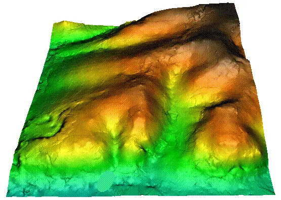
Ordinary Kriging Interpolation
Related Topics
Types of Interpolation Methods Choosing the Right Interpolation Method
References
University of the Western Cape
ESRI Education Services
IDRRE – Institute for Digital Research and Education
Kriging Interpolation by Chao-yi Lang, Dept. of Computer Science, Cornell University
Pollution models and inverse distance weighting: Some critical remarks by Louis de Mesnard
Overview of IDW – Penn State University


They are very useful guide. It is more complete if it comprises the nine interpolation methods and supported by video